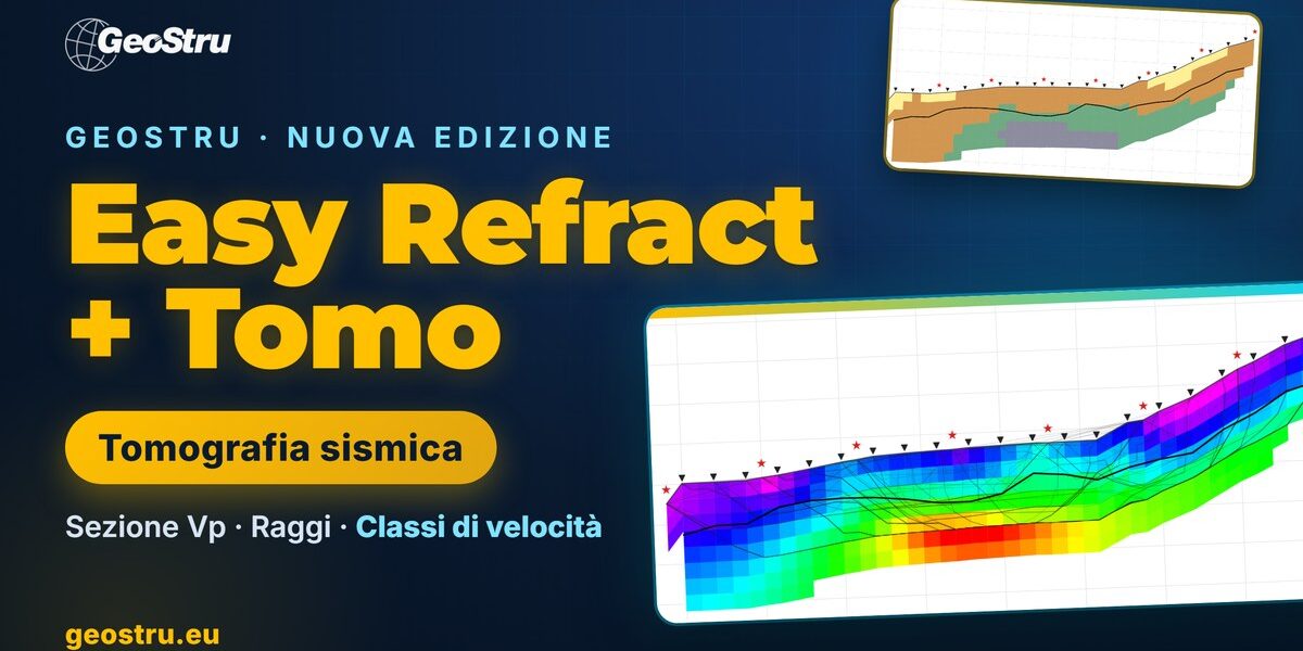
A seismic refraction survey interpreted with the classic methods gives a layered model: two or three refractors, each with its velocity and its depth below every geophone. That works well when the ground really is layered. But real ground has bedrock troughs, lenses of different material, weathering mantles that thicken, fractured zones along a fault. Seismic refraction tomography exists to see exactly these things: from the same first arrivals it builds a continuous velocity section, cell by cell, instead of a layered model. This article explains what it is, why it is done, how the data are acquired, how the computation works and how to read the result, using the new Easy Refract + Tomo edition by GeoStru as the example.
What seismic refraction tomography is
Seismic refraction tomography (SRT) is a geophysical method that reconstructs the distribution of seismic wave velocity in the ground along a vertical section. The data are those of an ordinary refraction survey: a line of geophones (the spread), a series of shots (sledgehammer, weight drop or other sources) and, for each shot and each geophone, the first-arrival time of the wave.
The difference lies in the interpretation. The ground is divided into a grid of cells, each with its own velocity. An algorithm searches for the velocity distribution that, propagating waves from the sources to the geophones, reproduces the measured times within the picking error. The result is a colour image of velocity — usually P-wave velocity (Vp) — that follows the topography and shows both vertical and lateral variations.
The term “tomography” comes from medicine: just as a CT scan rebuilds the inside of the body from many X-ray measurements along different paths, seismic tomography rebuilds the ground from many travel times along crossing seismic rays.
Why it is done: the limits of layered models
The classic refraction interpretation methods — the intercept-time method, the reciprocal method and Palmer’s Generalized Reciprocal Method (GRM) — are fast, robust and remain the standard for many geotechnical surveys. They rely, however, on a few assumptions:
- the ground is made of layers separated by sharp interfaces;
- velocity increases with depth from one layer to the next;
- within each layer velocity is constant, or varies little laterally.
When these assumptions fail, the layered model oversimplifies. A layer slower than the one above (velocity inversion) produces no refractor and stays invisible; a thin layer may never appear as a first arrival (hidden layer); a gradual velocity increase with depth, typical of soils that become denser or rock passing from weathered to sound, has no interface to pick. Above all, lateral variations — a bedrock trough, a lens, a fractured zone — are smeared over a layer with an average velocity.
Tomography does not need these assumptions: it does not ask how many layers there are or where they lie. That is why it is used when heterogeneous ground is expected, or to check the layered interpretation with an independent method.
Typical applications
- Landslides and unstable slopes: thickness of the debris cover or landslide body, shape of the stable bedrock, loosened zones. These data go straight into the geological model for slope stability analyses.
- Depth and shape of bedrock for foundations, retaining structures and excavations: troughs, steps, buried channels.
- Rippability of soil and rock: earth-moving equipment manufacturers’ charts relate Vp to ripping or to the need for breakers or blasting.
- Faults and fractured zones, which appear as low-velocity zones in the bedrock.
- Cavities, sinkholes and dissolution zones, as low-velocity anomalies (with the resolution caveats discussed below).
- Tunnel portals, dams and levees, landfills and contaminated sites, where a continuous section along the structure is needed.
- Hydrogeology: Vp rises to about 1500 m/s in saturated ground, and tomography helps locate the water table in loose deposits.
How the data for a tomography are acquired
The equipment is the same as for refraction: multichannel seismograph, vertical geophones (for P waves) or horizontal ones (for SH waves), a source. What changes most is the number of shots. Tomography needs many rays crossing the ground from different directions, so:
- frequent shots: besides the end and centre shots of classic refraction, one shot every few geophones along the spread (every 2–4 geophones is a good rule);
- off-end shots, beyond the outermost geophones: without them, bedrock depth at the edges of the section is constrained by few rays;
- geophone elevations surveyed carefully: topography enters the computation;
- accurately picked first arrivals on all shots, with an estimate of the picking error, typically 0.5–2 ms.
Depth of investigation depends on the spread length and on the velocity contrast; as an order of magnitude it is about one third to one quarter of the length. A spread of 24 geophones at 3 m (69 m) usually investigates the first 15–25 m. Resolution depends on geophone spacing and ray density: anomalies smaller than the geophone spacing cannot be resolved.
Good news: anyone with an archive of multi-shot refraction surveys can often reprocess them as tomography without going back to the field. With 5 shots and 12 geophones the result will be smooth and shallow, but it already shows the lateral variations that the layered model hides.
How the computation works
A refraction tomography alternates two problems.
The forward problem: given a velocity model, compute the arrival times at every geophone. The travel time T satisfies the eikonal equation |∇T| = 1/v, which says that the wavefront advances everywhere at the local velocity. The most widely used method for solving it on a grid is Fast Marching (Sethian, 1996): it propagates the front from the source cell by cell, in order of increasing time, and finds the fastest path by itself, whether a direct wave, a refracted wave or a wave going around an anomaly.
The inverse problem: correct the model to reduce the difference between computed and measured times. The problem is linearised around the current model (Gauss-Newton method) and a large sparse least-squares system is solved with iterative algorithms such as LSQR (Paige and Saunders, 1982). Since the data are fewer than the unknowns and contain errors, a regularisation is added: a smoothness constraint which, among all models compatible with the data, prefers the simplest one.
The two steps are repeated until the root-mean-square misfit (RMS) between measured and computed times drops to the level of the picking error. Going further makes no sense: it would mean fitting the model to the picking noise. Together with the section you get the ray coverage, which tells you in which cells velocity is actually constrained by the data.
How to read a tomographic section
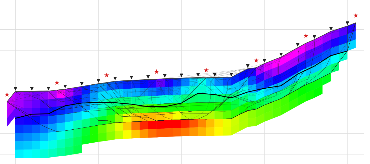
Three reading rules avoid the most common mistakes.
- Look at the rays. Where rays are dense and cross from different directions, velocity is well defined. At the edges and at depth, where rays are few or absent, the section mostly shows the starting model: read it with caution or hide it.
- Tomography smooths contrasts. The smoothness constraint turns a sharp boundary between two layers into a transition band. To place an interface, use a carefully chosen velocity contour, or compare with the layered interpretation.
- Velocity is not lithology. The section tells you how fast waves travel, not what the material is. It must be calibrated with boreholes, outcrops and site geology.
To read the section by zones, velocity classes are used. Indicative values for P waves:
| Vp [m/s] | Indicative interpretation |
|---|---|
| up to 800 | Cover, made ground, dry loose deposits |
| 800 – 1500 | Dense deposits, highly weathered rock |
| 1500 – 2000 | Saturated soils, weathered or fractured rock |
| over 2000 | Bedrock |
Beware of water: below the water table Vp exceeds about 1500 m/s even in loose soils, which may fall into the weathered-rock class. This is one reason why, where groundwater is present, P-wave tomography is best combined with a shear-wave survey.
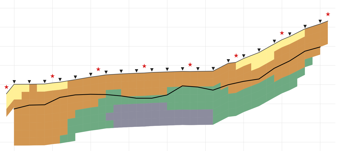
P-wave tomography and ground type
A useful note for those writing geological and geotechnical reports: seismic ground-type classification (Eurocode 8 and the Italian NTC 2018, § 3.2.2) is based on the equivalent shear-wave velocity (Vs,30 or Vs,eq), not on Vp. A P-wave tomography does not provide it. For Vs, surveys such as MASW, the HVSR spectral ratio or SH-wave refraction (which can also be processed as tomography, with velocity classes suited to S waves) are used. In practice the surveys complement each other: P-wave tomography describes the geometry of the ground along the section, MASW and HVSR give the Vs profile. We covered this in the article on joint MASW and HVSR analysis.
Tomography or GRM? A comparison
| Layered interpretation (GRM) | Seismic tomography | |
|---|---|---|
| Model | Layers with sharp interfaces | Grid of cells, continuous velocity |
| Lateral variations | Limited, interface by interface | Yes, including gradual ones |
| Vertical gradients | No (constant velocity per layer) | Yes |
| Velocity inversions | No | Partly (zones with poor ray coverage) |
| Sharp contrasts | Well defined | Smoothed into a transition band |
| Data required | Few shots (even 2–5) | As many shots as possible, including off-end |
| Typical result | Refractor depths and velocities | Vp section with ray coverage |
The two methods do not exclude each other; they complement each other. Overlaying the GRM refractors on the tomographic section is the simplest way to see whether the two readings agree and where the ground departs from the layered model.
Easy Refract + Tomo: tomography inside the refraction software
Easy Refract is GeoStru’s software for interpreting seismic refraction surveys: import of seismograms (SEG2, SEGY, SU and other formats), first-arrival picking, travel-time curves, intercept-time, reciprocal and GRM methods, automatic report. The new Easy Refract + Tomo edition includes all of Easy Refract and adds the Seismic tomography tab.
Its key strength is that nothing new has to be entered: spread geometry, geophone elevations and first arrivals of all shots are the ones already used for the interpretation. Open the tab, press Compute.
What it does
- Grid that follows the topography, with cell size and depth set automatically (one quarter of the geophone spacing, 35% of the spread length) or by hand.
- Travel times with the Fast Marching method and least-squares inversion (Gauss-Newton, LSQR) with a smoothness constraint that is gradually relaxed during the computation.
- Stops at the picking error (normalised chi-square equal to 1): the program does not fit the model to noise.
- Three starting models: automatic from the data (recommended), gradient, or from the GRM layered model.
- Background computation with live iteration and RMS; the program stays usable.
- Seismic rays, hidden ray-free zones, overlaid GRM interfaces, geophones and sources.
- Velocity classes with customisable limit, description and colour.
- Export of the section as an image, an XYZ grid (x, elevation, depth, velocity, ray coverage: opens in Surfer or a spreadsheet) and DXF with coloured cells, surface, interfaces and legend on separate layers.
- Dedicated chapter in the calculation report: method, parameters, fit quality, section image.
- The tomography is saved in the
.rftproject file, which remains readable by earlier versions of Easy Refract.
The workflow, in six steps
- Import the shot seismograms and pick the first arrivals, as for refraction.
- Enter the geophone elevations (the topography).
- Turn on the tab with Project > Process > Seismic tomography.
- Keep the default parameters, suitable for most cases, and press Compute.
- Check the final RMS (close to the picking error) and the ray coverage; compare the section with the GRM refractors.
- Turn on the velocity classes, export to DXF or XYZ and print the report.
The examples folder contains a real survey with 8 shots and 21 geophones, with topography, and the tomography already computed: RMS drops from about 6 ms for the starting model to about 1 ms. The computation on this example takes less than a second.
A validated, documented computation
Before release, the computation engine went through a validation with tolerances fixed in advance: computed times compared with closed-form solutions (homogeneous half-space, two layers, linear gradient, dipping refractor, sloping surface), a synthetic “bedrock step with fault” model based on the SAGEEP 2011 blind test (Zelt et al., 2013), with and without noise, and a comparison with a commercial tomography program on the same data. The results, including the cases where tolerances were not met and why, are collected in a public dossier on the GeoStru calculation code validation page. The validation also produced the most important practical advice: shoot beyond the ends of the spread.
Prices, upgrade and trial version
Easy Refract + Tomo is a single edition with a perpetual licence at €990 + VAT (Standard licence; Professional, Enterprise and Public Administration editions are available for companies, public bodies and resellers). Existing Easy Refract users can move to the new edition with a dedicated upgrade offer: contact the GeoStru sales office for the terms. The trial version includes tomography, with a “trial version” watermark on the section.
The tab’s manual is online: Seismic tomography – Easy Refract manual. For an overview of all GeoStru geophysics and geology programs, see our guide to the best software for geologists.
Discover Easy Refract + Tomo on the product page →
Frequently asked questions
It is a geophysical method that derives, from the first-arrival times of a refraction survey, a continuous section of seismic wave velocity, cell by cell, instead of a layered model. It shows gradual and lateral velocity variations: bedrock troughs, lenses, weathered or fractured zones.
The field data are the same; the interpretation changes. Conventional methods (intercept-time, reciprocal, GRM) assume layers of constant velocity increasing with depth and return refractor depths and velocities. Tomography assumes no layers: it divides the ground into cells and searches for the velocity distribution that reproduces the measured times. It sees gradients and lateral variations but smooths sharp contrasts. The two methods are used together.
The more shots, the better the result: besides the end and centre shots, one shot every 2-4 geophones and at least one off-end shot on each side are advisable. Easy Refract + Tomo warns when there are fewer than 5 shots or fewer than 100 first arrivals: the computation can still be run, but the section will be smooth and shallow.
As an order of magnitude, one third to one quarter of the spread length, depending on the velocity contrast and on shot positions. A spread of 24 geophones at 3 m usually investigates the first 15-25 m. Ray coverage shows how deep the section is constrained by the data.
Not P-wave tomography, which gives Vp. Ground-type classification (Eurocode 8, Italian NTC 2018) is based on shear-wave velocity, obtained from MASW, HVSR, down-hole or SH-wave refraction (which can also be processed as tomography). P-wave tomography describes the geometry of the ground well and complements these surveys.
Widely used programs include Rayfract, SeisImager/2D, ReflexW and, among open-source tools, pyGIMLi. GeoStru’s Easy Refract + Tomo combines first-arrival picking, GRM interpretation and tomography (Fast Marching and Gauss-Newton/LSQR inversion) in one program, with velocity classes, DXF and XYZ export, automatic report and a published validation. A trial version is available.
References
- Palmer D. (1980). The Generalized Reciprocal Method of Seismic Refraction Interpretation. Society of Exploration Geophysicists, Tulsa.
- Sethian J.A. (1996). A fast marching level set method for monotonically advancing fronts. Proceedings of the National Academy of Sciences, 93(4), 1591–1595.
- Paige C.C., Saunders M.A. (1982). LSQR: An algorithm for sparse linear equations and sparse least squares. ACM Transactions on Mathematical Software, 8(1), 43–71.
- Sheehan J.R., Doll W.E., Mandell W.A. (2005). An evaluation of methods and available software for seismic refraction tomography analysis. Journal of Environmental and Engineering Geophysics, 10(1), 21–34.
- Zelt C.A., Haines S., Powers M.H., et al. (2013). Blind test of methods for obtaining 2-D near-surface seismic velocity models from first-arrival traveltimes. Journal of Environmental and Engineering Geophysics, 18(3), 183–194.