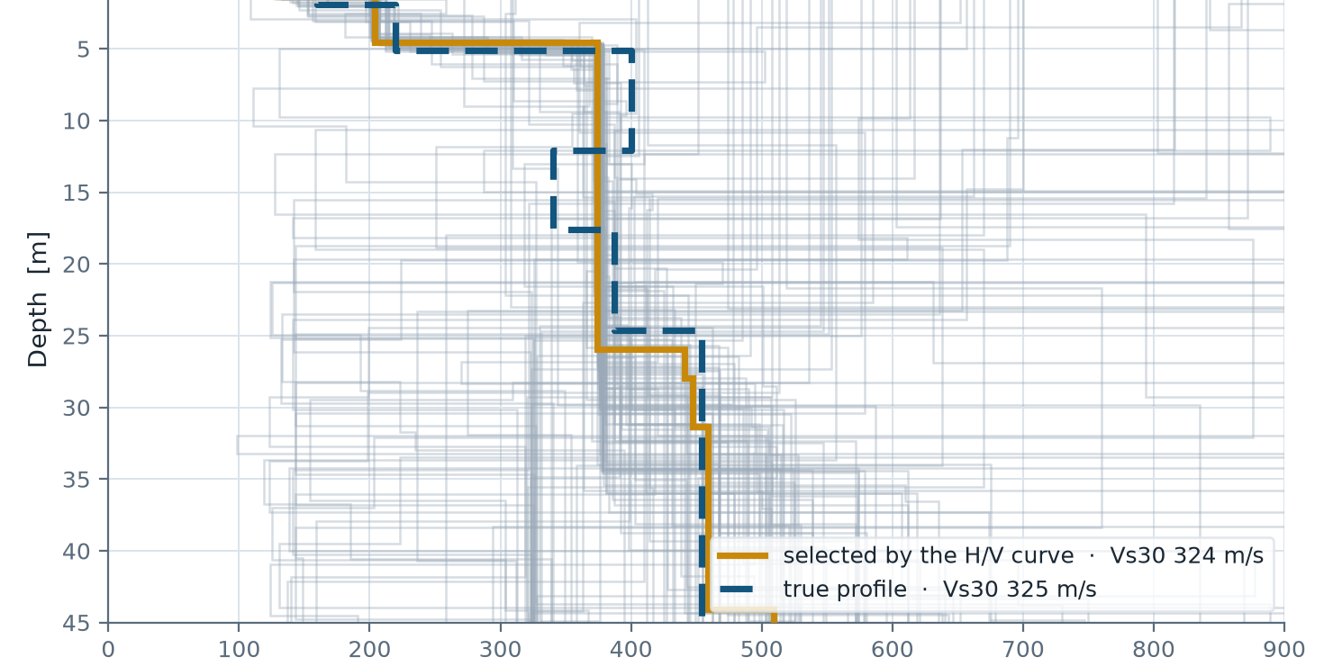
Every geophysical technique suffers from non-uniqueness: many different subsoil models are compatible with the same measurement. This is not a shortcoming of the instruments, it is a property of the information the measurement carries. We set out to measure how much it really weighs, and the result surprised us.
The experiment
We started from a known subsoil profile, eight layers, with a Vs30 of 325 m/s. From that profile we generated the dispersion curve a MASW survey would have measured. Then we pretended not to know the answer and worked backwards: from the data, reconstruct the ground. Two hundred times, with different initial assumptions.
The advantage of working this way is that we know the right answer. With field data you can never tell whether the profile you obtained is the true one; here you can, and the error can be measured.
One hundred and twenty-two profiles, all “correct”
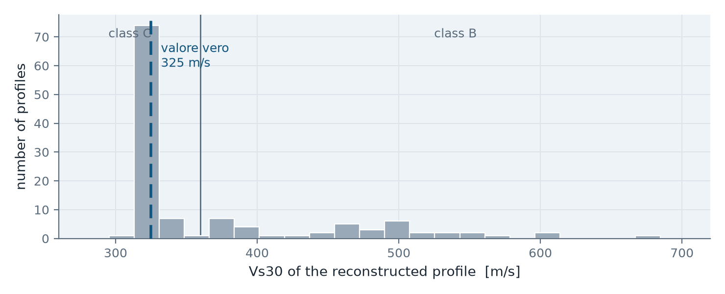
Out of 200 attempts, 122 produced a profile explaining the dispersion data with an error below 3%: a fit any operator would consider excellent.
Those 122 profiles are not variations on a theme. They are different profiles:
- the lowest has Vs30 = 300 m/s
- the highest has Vs30 = 679 m/s
The boundary between class B and class C — 360 m/s — falls in the middle of the distribution: 83 profiles fall in class C, 39 in class B. One profile in three, from identical data, leads to a different seismic classification.
This is the point that usually remains unspoken: when software returns one profile, it is not saying the others are wrong. It is saying that it has stopped searching.
What happens when you add the H/V curve
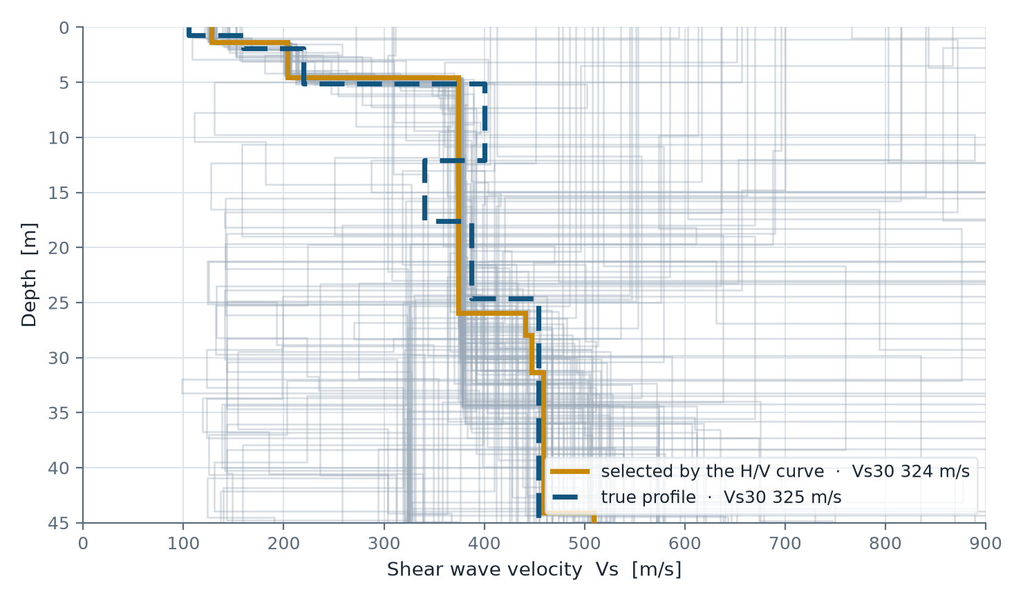
We took those 122 profiles — all indistinguishable on the basis of dispersion alone — and asked each of them to explain also the H/V curve measured at the same point with a three-component tromometer.
The profile that explains it best has Vs30 = 324 m/s. The true value was 325 m/s.
This is not a marginal improvement: it is the step from a problem with hundreds of solutions to a problem with one. The H/V curve alone would not have been enough to reconstruct the profile — but it is exactly the information MASW is missing in order to be decisive.
The H/V curve tells you where the bottom is. MASW dispersion tells you what lies above it. Neither of them, on its own, tells you both.
The limit almost nobody states: the spread length
There is a second, even more practical aspect, which emerged while working on a real case.
A MASW survey reliably resolves wavelengths of the order of the spread length. Each picked point, at frequency f and phase velocity v, corresponds to a wavelength λ = v/f, and the investigated depth lies roughly between λ/3 and λ/2.
| Spread length | Depth actually investigated | Vs30 determinable? |
|---|---|---|
| 24 m | 8–12 m | no, largely extrapolated |
| 48 m | 16–24 m | partly |
| 72 m | 24–36 m | yes |
The comparison with the 30 metres required by Vs30 is immediate: with short spreads the deeper part of the profile is not measured, it is extrapolated. And that is precisely the portion the H/V curve, which measures the resonance of the whole column, is able to constrain.
In a real case with a 24-metre spread, two points had been picked at 4.7 and 5.0 Hz with velocities of 491 and 428 m/s: wavelengths of 104 and 85 metres, more than four times the spread. To explain them, the inversion placed a 717 m/s substratum at 18 metres depth — a bedrock that does not exist. The fit remained excellent and no indicator flagged the problem. Once those two points were removed, the conflict disappeared.
The error that leaves no trace
Finally, there is an error that happens in the field, and it is invisible. In the velocity spectrum one identifies a well defined curve and interprets it as the fundamental mode. Sometimes it is not: when energy spreads onto the higher modes, the fundamental can be weak or entirely absent, and the most visible curve is in fact a higher mode.
In our tests, attributing to the fundamental a curve that was instead the first higher mode shifted the Vs30 from 325 to 451 m/s: a wrong subsoil class, with a dispersion fit error below 1%. Repeated 155 times, the error proved systematic — always in the same direction, never random.
A mode misinterpretation does not produce uncertainty. It produces a wrong answer, precise and consistent.
How it is done, in practice
- In the field: at the same point, the usual MASW spread and a 15–20 minute HVSR recording with a three-component tromometer, preferably at the centre of the spread.
- In Easy MASW: pick the dispersion curve, assigning its own mode number to each curve, and export the modal curves.
- In Easy HVSR: import the dispersion and run the joint inversion. A single Vs profile, consistent with both measurements.
What to take away
- A low misfit does not certify the result. It says the model is compatible with the data, not that it is the only one. The right question is: how many other models get there too?
- MASW alone is an under-determined problem. It is not a limitation of the software: it is a property of the data. No algorithm can recover information the measurement does not contain.
- An HVSR recording at the same point costs fifteen minutes, and it is the missing information. The ratio between acquisition cost and uncertainty reduction is probably the best available in applied near-surface geophysics.
- The mode must be identified, not assumed. A “clean” spectrum is not automatically a fundamental mode.
- Beware of values close to class boundaries. 360 m/s separates B from C: a result of 350 or 380 m/s obtained from a single method is a design decision resting on an uncertainty that has never been measured.
A methodological note
The figures in this article come from synthetic data: known profile, computed curves, no instrumental noise. This is a deliberate choice — only this way is the exact answer known and the error measurable.
With real data the situation is harder, not easier: noise, three-dimensional effects, H/V peaks of anthropic origin. The non-uniqueness measured here is therefore an optimistic estimate.
Joint MASW + HVSR analysis is available in Easy MASW and Easy HVSR. A complete technical guide, with the step-by-step procedure and practical advice for the inversion, can be downloaded as a PDF: Joint MASW + HVSR analysis — guide.
Online manuals: help.geostru.io/masw · help.geostru.io/easyhvsr