Liquefaction resistance of soil with Liquiter

Simplified procedure for evaluating liquefaction resistance of soils

Following disastrous earthquakes that occurred in Alaska and Niigata (Japan in 1964), Seed and Idris (1971) proposed a simplified methodology for assessing the resistance to liquefaction of soils. This methodology has been selected and improved over the years (e.g. Seed, 1979; Seed and Idriss, 1982; Seed et al., 1985) become a widely used standard and reference for liquefaction hazard assessment (NRC 1985). Updates to the simplified procedure were discussed in a seminar by Youd and Idriss (1997) and published in the report “Liquefaction Resistance of Soils” (Youd and Idriss, 2001).

These updates are included in Liquiter software (Fig.1).

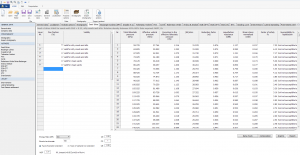
Fig. 1 – In this section of Liquiter several methods are reported

The simplified procedure is developed on the basis of empirical evaluations of in situ and laboratory tests. In the first case, SPT, CPT, geophysical surveys are carried out. Field evidence of liquefaction generally consisted of surficial observations of sand boils, ground fissures, or lateral spreads. In the second case the methods are based on the shear strength tests and triaxial tests.

The phenomenon of liquefaction

Liquefaction is a phenomenon that occurs when a soil, subjected to a seismic shock, shows an increase in interstitial pressures and a zero shear resistance. The change in physical state (from solid to liquid) generally occurs on saturated granular material surface deposits with characteristics that cannot dissipate the interstitial pressure with sufficient speed following an earthquake.

As shown by Mohr Coulomb‘s equation, the shear strength (τ) tends to decrease due to the cancellation of the effective tension (σ ’= σ-u):

τ = (σ-u) tgφ + c

with σ = total normal voltage; u = interstitial pressures φ = friction angle and c = cohesion.

So if u increases to equal σ, the effective pressure is canceled and the resistance tends to zero, thus determining the liquefaction condition.

CSR and CRR

To determine the risk of liquefaction in terms of safety factor (FS), the calculation of two variables is required: 1) CSR= Cyclic Shear Ratio and 2) CRR Cyclic Resistance Ratio.

The simplified methods are based on the relationship between the shear stresses which produce liquefaction and those induced by the earthquake; therefore they need to evaluate the parameters for both seismic event and deposit. The resistance to liquefaction of the deposit is then calculated in terms of liquefaction resistance factor.

Criteria for evaluation of liquefaction resistance based on SPT

The method of Seed e Idriss (1982) calculates the CSR using the following formula:

CSR=τ_av/(σ_v0^’ )=0.65∙(a_max/g)∙(σ_v0/(σ_v0^’ ))∙r_d

The value r_d is the stress reduction coefficient and is determined as follows (Liao e Whitman,1986):

r_d=1.0-0.00765z per z≤9.15m
r_d=1.174-0.0267z per 9.15m<z≤23m

Where z is depth below ground surface in meters.

For Magnitude 7,5 Earthquakes the original curve of Seed and Idriss (1982) is considered (Fig.2).

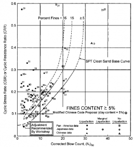
Fig. 2 – SPT Clean Sand-Base Curve for Magnitude 7.5 Earthquakes (mod. from Seed et al., 1985)

The formula is:

CRR_7.5=1/34-(N_1)_60 +(N_1)_60/135+ 50/[10∙(N_1)_60+45]^2 – 1/200

This equation is valid for N1(60)<30. For N1(60)≥30, clean granular soils are too dense to liquefy and are classed as “non-liquefiable”.

For different Magnitude (greater or less than 7.5) Seed e Idris (1982) introduced the Magnitudo Scaling Factor MSF defined by the following equation:

MSF= 10^2.24/(M_w^2.56 )

A set of magnitude scaling factor M_w are listed in Table1.

Table 1– Scale factor of the magnitude derived from several researchers

Magnitude	Seed H.B. & Idriss I.M. (1982)	Ambraseys N.N (1988).	NCEER (Seed R. B. et all) (1997; 2003)
5,5	1,43	2,86	2,21
6,0	1,32	2,20	1,77
6,5	1,19	1,69	1,44
7,0	1,08	1,30	1,19
7,5	1,00	1,00	1,00
8,0	0,94	0,67	0,84
8,5	0,89	0,44	0,73

The Cyclic Resistance Ratio is calculated as a function of magnitude, the number of blows in the SPT test, the effective vertical pressure and the relative density.

At first, the corrected number of blows count is calculated:

(N₁)_60CS= α+β(N₁)₆₀

where α e β are coefficients reported in Table2:

FC	α	β
≤5%	α = 0.0	β=1.0
5%<FC≥35%	α=exp[1.76-(190/FC2)]	β= 0.99+(FC1.5/1000)
FC≥35%	α = 5.0	β=1.2

Table 2– Influence of Fine Content (FC)

Other corrections that influence SPT results are incorporated in these corrections:

(N₁)₆₀ =N_mC_NC_EC_BC_RC_S

where N_m is the measured standard penetration resistance; C_N is a correction factor to normalize N_m to a common reference effective overburden stress; C_E is the corretion for hammer energy ratio (ER); C_B is the correction factor for borehole diameter; C_R is the correction factor for rod length; and C_S is the correction for samples with or without liners.

Factor of safety

To illustrate the influence of magnitude scaling factors on calculated hazard, the equation for factor of safety (FS) against liquefaction is written in terms of CRR, CSR, and MSF as:

FS= (CRR_7.5/CSR)MSF

where CSR is the calculated cyclic stress ratio generated by the earthquake shaking; and CRR7.5 is the cyclic resistance ratio for magnitude 7.5 earthquakes.

Software

Considering the text described above the use of the following softwares are recommended:

• Liquiter – software is designed for soil liquefaction analysis and supports a wide variety of field tests.
• DYNAMIC PROBING – Dynamic penetration tests – Software used for Dynamic Penetration Tests, that is the reading, recording, interpretation, storage and the management of any type of penetrometer including new or custom equipment and of in borehole SPT readings.
• STATIC PROBING – Static penetration tests – This program processes and archives penetrometric equipment readings for static penetrometers such as CPT (Cone penetration test), CPTE (Cone penetration test electric) and CPTU (Cone penetration test Piezocone).

Geoapp

Geostru company created a service available on the Geoapp web page where there are several applications for making online calculations. Geoapp includes over 40 applications for: Engineering, Geology, Geophysics, Hydrology and Hydraulics.
Among the applications present, a wide range can be used together with the software mentioned above, for example:

•  Sismogenetic zone
•  Soil classification SMC
• Seismic parameters
• NSPT
• Slope stability
• Landslide trigger
• Critical heigh (maximum depth that can be excavated without failure)
• Bearing capacity
• Lithostatic tensions
• Foundation piles, horizontal reaction coefficient
• Liquefaction (Boulanger 2014)

Courses

Soil liquefaction and stabilization

References

Castro, G. (1995). ‘‘Empirical methods in liquefaction evaluation.’’ Primer Ciclo d Conferencias Internationales, Leonardo Zeevaert, Universidad Nacional Autonoma de Mexico, Mexico City.

Seed, H. B. (1979). ‘‘Soil liquefaction and cyclic mobility evaluation for level ground during earthquakes.’’ J. Geotech. Engrg. Div., ASCE, 105(2), 201–255.

Seed, H. B., and Idriss, I. M. (1971). ‘‘Simplified procedure for evaluating soil liquefaction potential.’’ J. Geotech. Engrg. Div., ASCE, 97(9), 1249–1273.

Seed, H. B., and Idriss, I. M. (1982). ‘‘Ground motions and soil liquefaction during earthquakes.’’ Earthquake Engineering Research Institute Monograph, Oakland, Calif.

Seed, H. B., Tokimatsu, K., Harder, L. F., and Chung, R. M. (1985). ‘‘The influence of SPT procedures in soil liquefaction resistance evaluations.’’ J. Geotech. Engrg., ASCE, 111(12), 1425–1445.

Youd and Idriss, I. M. (2001). Liquefaction resistance of soils: summary report from the 1996 NCEER and 1998 NCEER/NSF workshops on evaluation of liquefaction resistance of soils. Journal of geotechnical and geoenvironmental engineering.